Excel tips and tricks (v10, May 2024)
19-May-24: Added section for Named ranges.
18-May-24: Added section for calling subs.
20-Apr-24: Added explanation of the UsedRange.
20-Apr-24: Added a UserForm to show Row&Col nr of selected cell
06-Jan-24: Added a progress bar.
06-Jan-24: Added a sleep method to the timer class.
Contents
- Using a class for persistent public variables
- Measure the execution time of code
- Speed up execution of VBA code / macro
- Show progress in code execution in a progress bar
- Store the value of a forms controls (i.e. checkbox or textbox) between sessions
- Position of (pop-up) window on the screen and worksheet
- Using arrays to speed up read and write to worksheet cells
- Adding a menu to the ribbon
- Making your own custom functions
- The difference between HIDE and UNLOAD of a form
- Events triggered by the form controls
- Regular expressions with user defined functions
- Reading table filter settings
- Working with the UsedRange
- UserForm to show/goto row & col nr
- Calling subs from worksheets and modules
- Named ranges in VBA
Using a class for persistent public variables
In excel VBA it is good practise to define variables on the lowest possible level. So within subs or functions. But sometimes it is useful to deine a variable on global workbook scope. In my excel code I make use of arrays to read and write to sheets. These are used throughout the sheets and modules. Or you have a workbook wide variable like 'DebugMode'. When this is TRUE the subs in the workbook print information in the immediate window and event handling is different. I declare these public global variables in a module. Another example is a variable to keep track of the last line of a dynamic table in an excel sheet. For instance in a module I call "InitPublics" there is a line:
dPublic LastRowOfTable as IntegerThe problem I faced with this is that these variables looses their value once the code is interrupted by a run time error. Especially for testing this is a pain. When you use a public constant such as:
Public LastRowOfTable as Integer = 10Then the value will not be 'lost' during run time error but if the length of the table changes you cannot change the value of the constant during runtime.
A possible solution for this is to use a class property as a (public) variable. The advantage of a class property is that it has GET and LET methods that are activated during reading and writing of the property. You can use these methods to manipulate the value of the variable. Another great advantage is that you can create dynamic constants. Meaning that a variable can be read only for the code. Only within the class the variable gets a value. So the class does not prevent that variable values are lost during runtime errors but it can initialize the variables before they are actually used. Once you know how to do this, then working with these classes is quite simple. As a demonstration you can have the following code in your project in a class module named ClassGlobalVariables:
Private pDemoReadProperty As Integer
Private pDemoReadWriteProperty As Integer

' DemoReadProperty
Public Property Get DemoReadProperty() As Integer
	If pDemoReadProperty > 0 Then pDemoReadProperty = pDemoReadProperty - 1
	If pDemoReadProperty = 0 Then pDemoReadProperty = 10
	DemoReadProperty = pDemoReadProperty
End Property

' DemoReadWriteProperty
Public Property Get DemoReadWriteProperty() As Integer
	If pDemoReadWriteProperty = 0 Then pDemoReadWriteProperty = 100
	DemoReadWriteProperty = pDemoReadWriteProperty
End Property
Public Property Let DemoReadWriteProperty(val As Integer)
	pDemoReadWriteProperty = val
End Property
For demo purposes there are only 2 variables. One that is read only and one that is read write. The GET procedure is activated when the value of the variable is read in the code. The LET procedure is activated when the variable is set in the code. As you can see the read property only has a GET method. In the GET method of the read only property the value is set to 10 when it is not initialized yet. This sets the variable during first use in the code but also resets it if the value is lost during a run time error. As a demo I have added a line where the value of the read only variable is decremented by 1 every time the variable is read in the code.
Public GlobalVar As New ClassGlobalVariables

Sub DemoGlobalVars()

Dim i As Integer
Dim c As String

' read inital value of read only property
i = GlobalVar.DemoReadProperty

' read changed value read only property
i = GlobalVar.DemoReadProperty

' next line creates a run time error causing variables to loose their values
On Error Resume Next
i = i * c
On Error GoTo 0

' read again inital value of read only property
i = GlobalVar.DemoReadProperty

' read inital value of read and write property
i = GlobalVar.DemoReadWriteProperty

' next line will give a compiller error "Can't assign to read only property". Remove the comment to check this:
GlobalVar.DemoReadProperty = i - 1

' this sets the read write property
GlobalVar.DemoReadWriteProperty = i - 1

End Sub
When using the variables in your code you have to prefix the variable name with the name GlobalVar followed by a dot. Excel will give you a drop down of the defined properties during typing so that it is quicker to enter and less chances of typos. The first attempt to read the value of the read-only variable will result in the initial value of 10 for i. In the next attempt i will be 9 because it is decremented in the GET method. An attempt in the code to assign a value to a read only variable will result in a compiler error.
Time the exection of code
To measure the execution speed of a piece of code is simple. You set a variable to the time value before you run the code and immediately after. The difference between the two is the time it took to execute the code. Simple enough, but there is a problem. The problem is that the default and only VBA function to return a time value =Time() has a resolution / granularity of seconds. So measuring anything smaller than a second is not possible. Therefore Microsoft published code called MicroTimer to produce a time value with a micro second granularity.
Based on this code I made a so-called class named ClassTimer to define some methods to easily do this time measurement. The class enables you to use Timer.Start before the code under test and Timer.Finish after the code under test to print the execution time. In the class I convert the MicroTimer to milliseconds because for me that is enough. And the execution time of the Timer class subs would be negligable. For fast code I execute it in a loop of 1000x-1000000x to produce readable results. Together with the statements to disable events (see next section about speeding up code) the VBA code for testing execution time becomes:
Dim Timer As New ClassTimer
Application.ScreenUpdating = False
Application.EnableEvents = False
Application.Calculation = xlCalculationManual
Application.Cursor = xlWait ' to reduce cursor flicker and improve speed of code

Timer.Start "Timer demo ..."
For i = 1 To 1000
	'
	"place code to test here"
	'
Next i
Timer.Finish

Application.Cursor = xlDefault
Application.ScreenUpdating = True
Application.EnableEvents = True
Application.Calculation = xlCalculationAutomatic
The result is written by the ClassTimer to the immediate window in the VBA editor using the command Debug.Print. It looks something like:
05/01/2024 15:32:57 === Timer demo ...
0,665         = Total from start
The first line with the time value is written by the timer.Start method. It can optionally print an additional text. This method set the internal timer to 0. The Timer.Finish method prints the internal timer.
This class also has some more methods:
Timer.Inter: To display the running timer without resetting it to zero. This could be used as intermediate checkpoints for larger bits of code, where you also want to know to total time for all the code.
Timer.Restart: To display the running timer value. This also resets the timer. This is basically the samea as timer.Inter followed by Timer.Start
Timer.Sleep: This creates a delay in mSec. It uses the same microtimer() but this time to create a delay. The accuracy of the delay is +0 to +1 mSec from the given value. The given value can be a fraction, e.g. 2.5 mSec. Long delays can be interrupted with the Ctrl-Break key combination. It turns out that when used in a loop the overall accuracy remains +0 to +1 mSec. So using Timer.Sleep 1 in a loop of 1000 itterations still has an overall of 1.000 - 1.001 Sec delay. Of course, assuming there is no other code in the loop. This delay is more accurate then the sometimes used API call Public Declare PtrSafe Sub Sleep Lib "kernel32". For more explanation of the actual measured delay times of the API Sleep call, see 'Module7_Sleep' in the sample excel file.
Speed up execution of VBA code / macro
To speed up the execution of code that manipulates cells in worksheet and also to reduce screen flickering during code execution, I put the following lines before and after the code:
	Application.ScreenUpdating = False
	Application.EnableEvents = False
	Application.Calculation = xlCalculationManual
	Application.Cursor = xlWait
	Application.ScreenUpdating = True
	Application.DisplayStatusBar = True
	Application.StatusBar = "Message that code is executing..."

	< code to execute >

	Application.StatusBar = ""
	Application.Cursor = xlDefault
	Application.Calculation = xlCalculationAutomatic
	Application.EnableEvents = True
	Application.ScreenUpdating = True
Application.ScreenUpdating : Stops updating/refreshing the screen while the code is running. This is especially effective when the worksheet cells that are updated by the VGA code are visible for the user.
Application.EnableEvents : This prevents code is interrupted by events. Event could be something like changing a value of a cell. Remember that cells could be changed by the code and would trigger events like the Worksheet_Change() event.
Application.Calculation : To not trigger the calculation when cells are changed by the code. Remember that cells could be changed by the code also would trigger the calculation of the sheet.
Application.Cursor : This changes the cursor to a waiting circle. To reduce cursor flicker. Is also an indication to the user that code is executing and seems to speed up code execution.
Application.StatusBar : Displays a message in the left lower corner of the excel window. This does not actually improve the execution speed of the code but it can make it clear to the user that something is running. Current status is saved before message is displayed. Status bas is restored after code execution.
If code is stopped during execution e.g. by an error then the status of the events is not restored since these statement were not executed. This is especially anoying for the cursos which is still in the wrong state (circle) and the events are no longer executed. Therefore I leave out these lines until the code if fully debugged.
If code is called by other subroutines then it is better to store the current status and restore after code is executed:
	Dim currEnableEvents as Boolean
	Dim currScreenUpdating as Boolean
	Dim currCalculationMode as xlCalculation
	Dim oldStatusBar As Boolean

	currEnableEvents = Application.EnableEvents
	currScreenUpdating = Application.ScreenUpdating
	currCalculationMode = Application.Calculation

	Application.ScreenUpdating = False
	Application.EnableEvents = False
	Application.Calculation = xlCalculationManual
	Application.Cursor = xlWait
	oldStatusBar = Application.DisplayStatusBar
	Application.DisplayStatusBar = True
	Application.StatusBar = "Message that code is executing..."

	< code to execute >

	Application.StatusBar = ""
	Application.DisplayStatusBar = oldStatusBar
	Application.Cursor = xlDefault
	Application.Calculation = currCalculationMode
	Application.EnableEvents = currEnableEvents
	Application.ScreenUpdating = currScreenUpdating
Application.ScreenUpdating : Stops updating/refreshing the screen while the code is running.
Application.EnableEvents : This prevents code is interrupted by events. Event could be something like changing a value of a cell. Remember that cells could be changed by the code.
Application.Calculation : To not trigger the calculation when cells are changed by the code.
Application.Cursor : This changes the cursor to a waiting circle. To reduce cursor flicker. Is also an indication to the user that code is executing and speeds up code!!
Application.StatusBar : Displays a message in the left lower corner of the excel window. Current status is saved before message is displayed. Status bas is restored after code execution.
During code development I was interested in the parts of the code that contributred the most to the execution time of the code. Therefore I conducted some test on code snippets to measure the time needed. The absolute values of the measurements may vary from computer to computer depending on the exact version of Windows and maybe Excel and the hardware of the computer used. But the values can be compared to each other to determine which code is fast and which is slower. The measurements were done on Windows 11 and a processor 11th Gen Intel(R) Core(TM) i7-11700 @ 2.50GHz together with the built in graphics UHD 750. All measurements were done with the above mentioned method. Code snippets were executed 1x (Sec), 1000x (mSec) or even 1000000x (µSec).
The table below gives the execution times for the various ways of reading a value from a cell:
| Code Snippet | Time [µSec] | Remark |
|---|---|---|
v = ActiveCell.Value |
1 | Is fast but the select method needed to place the active cell takes long, see below |
v = Cells(1, 1) |
2 | This seems the fastest way to read a cell's value |
v = Range("A1") |
3 | |
v = Sheet8.Rows(1).Columns(1) |
3 | |
v = Sheet8.Range("A1") |
4 | Including sheet internal name adds additional execution time |
v = Range("A1:A1") |
4 | |
v = Range("NamedRangeA1") |
4 | |
v = Sheets("ExecTimes").Cells(1, 1) |
6 | Using the sheet tab name adds additional execution time |
Range("A1").Selectv = ActiveCell.Value |
30 | can increase >5x when ScreenUpdating = True |
Some measurements for reading other properties of a cell. All these have more or less the same execution time:
| Code Snippet | Time [µSec] | Remark |
|---|---|---|
v = Cells(1, 1).Interior.Color |
6 | background color as an RGB value |
v = Cells(1, 1).Font.Color |
5 | font color as RGB value |
v = Cells(1, 1).Font.Bold |
5 | bold value as TRUE/FALSE |
v = Cells(1, 1).NumberFormat |
5 | number format as string e.g. "[$-F400]h:mm:ss AM/PM" |
v = Cells(1, 1).ColumnWidth |
5 | |
v = Cells(1, 1).RowHeight |
5 |
The next table gives some values for writing to a cell:
| Code Snippet | Time [µSec] | Remark |
|---|---|---|
Cells(1, 4) = "" |
13 | Writing to a cell is much slower than reading, see table above. But using Cells(1,4) seems the fastest way to do it. |
Cells(1, 4) = 3 |
14 | |
Cells(1, 4) = "test" |
14 | |
Cells(1, 4) = String(1000, "h") |
19 | a long string of 1000 chars takes only a bit longer |
Cells(1, 4) = True |
14 | |
Cells(1, 4) = 1.23 |
14 | |
Range("D1") = "" |
19 | using Range("D1") is slower than using Cells(1,4) |
Range("D1:D1") = "" |
20 |
And some random VBA code functions, methods and snippets that I used in my code:
| Code Snippet | Time [µSec] | Remark |
|---|---|---|
v = CStr(i) |
0.05 | |
v = Format(i) |
0.1 | Very fast but slower than CStr() |
v = Format(i, "0.0") |
0.2 | Adding a parameter makes the time larger |
v = Instr(1,"string of 10x a char long","x") |
0.1 | Fast function to detect if one string exists in another. |
v = Instr(1,"string of 100x a char long","x") |
0.3 | Only slightly larger execution time for longer strings |
v = Instr(1,"string of 1000x a char long","x") |
1.2 | Still fast even for very long strings |
Set rng = Range(Cells(1, 1), Cells(10, 10)) |
2 | Assigning a range to a variable. The size of the range has little effect on the time. |
Set rng = Range("A1:CV100") |
2 | Assigning a range to a variable. The size of the range has little effect on the time. |
|
0.02 | Superfast |
|
0.016 | Even faster than select case but perhaps less elegant. |
|
6 | Execution time largely independent from range. |
|
1 | Using Row and Column is faster then using the intersect function. |
Execution times of the lookup functions:
| Code Snippet | Time [µSec] | Remark |
|---|---|---|
WorksheetFunction.XLookup("not found", Sheet8.Range("B1:B10"), Sheet8.Range("A1:A10")) |
12 | shorter if value found before end |
WorksheetFunction.XLookup("not found", Sheet8.Range("B1:B100"), Sheet8.Range("A1:A100")) |
14 | shorter if value found before end |
WorksheetFunction.XLookup("not found", Sheet8.Range("B1:B1000"), Sheet8.Range("A1:A1000")) |
24 | shorter if value found before end |
WorksheetFunction.XLookup("not found", Sheet8.Range("B1:B10000"), Sheet8.Range("A1:A10000")) |
120 | shorter if value found before end |
WorksheetFunction.XLookup("not found", Sheet8.Range("B1:B100000"), Sheet8.Range("A1:A100000")) |
1100 | shorter if value found e.g. 24 uSec if found at pos 1000 |
WorksheetFunction.Match("not found", Sheet8.Range("B1:B10"), 0) |
5 | exact match |
WorksheetFunction.Match("not found", Sheet8.Range("B1:B100"), 0) |
7 | |
WorksheetFunction.Match("not found", Sheet8.Range("B1:B1000"), 0) |
10 | shorter if value found before end |
WorksheetFunction.Match("not found", Sheet8.Range("B1:B10000"), 0) |
60 | shorter if value found before end |
WorksheetFunction.Match("not found", Sheet8.Range("B1:B100000"), 0) |
500 | shorter if value found, eg 10 uSec if found at pos 1000 |
WorksheetFunction.Index(Range("A1:A10"), WorksheetFunction.Match("Row10", Range("B1:B10"), 0)) |
11 | about the same as equivalent XLookUp function |
WorksheetFunction.Index(Range("A1:A100"), WorksheetFunction.Match("Row100", Range("B1:B100"), 0)) |
13 | shorter if value found before end |
WorksheetFunction.Index(Range("A1:A1000"), WorksheetFunction.Match("Row1000", Range("B1:B1000"), 0)) |
17 | shorter if value found before end |
WorksheetFunction.Index(Range("A1:A10000"), WorksheetFunction.Match("Row10000", Range("B1:B10000"), 0)) |
70 | shorter if value found before end |
WorksheetFunction.Index(Range("A1:A100000"), WorksheetFunction.Match("Row100000", Range("B1:B100000"), 0)) |
500 | shorter if value found, eg 17 uSec if found at pos 1000 Faster than equivalent XLookup() for large ranges! |
|
250 | Due to Cells() method, slower than equivalent match() function. |
The following table shows the difference in reading a range cell by cell in a for next loop or using an array to read a range. As you can see, using an array is much faster. Note that the values are in [mSec] now:
| Code Snippet | Time [mSec] | Remark |
|---|---|---|
shArr = Sheet8.Range(Cells(1,1),Cells(100,100)) |
0.25 | Dim shArr() as Variant |
|
18 | Dim shArr(1 to 100, 1 to 100) as Variant |
shArr = Sheet8.Range(Cells(1,1),Cells(1000,1000)) |
30 | Dim shArr() as Variant |
|
1700 | Dim shArr(1 to 1000, 1 to 1000) as Variant |
The following table shows the difference in writing a range cell by cell in a for next loop or using an array to write to the range. As you can see, using an array is much faster. I could not find a significant difference in writing to a cells/range .Value, .Value2, .Formula or .Formula2 property. Also the type of the array seem to have no affect. With the shArr defined as integer, string, single, date etc the same result was obtained. I made the array the same size as the range being written to but in reality the shArr can be bigger than the range:
| Code Snippet | Time [mSec] | Remark |
|---|---|---|
Range(Cells(1,1),Cells(100,100)) = shArr |
4 | Dim shArr() as Variant. shArr filled with numers 0 to 9999 |
|
130 | Dim shArr(1 to 100, 1 to 100) as Variant |
Range(Cells(1,1),Cells(1000,1000)) = shArr |
400 | Dim shArr() as Variant. shArr filled with numers 0 to 999999 |
|
12400 | Dim shArr(1 to 1000, 1 to 1000) as Variant |
Progress Bar
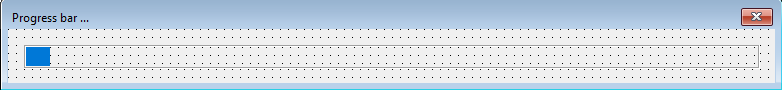
Made a small UserFormProgressBar to be able to show a progress bar when code execution takes a bit longer, more than a few seconds. The UserForm contains a colored rectangle that is changed in width to mimic the progress. The progress bar can handle a Min and an Max scale value and display the progress in between these. The progress bar is controlled with a few methods that are added to the code of the UserForm:
UserFormProgressBar.SetMinScale: To set the value belonging to the minimum of the progress bar, i.e. 0% progress. The default is 0.
UserFormProgressBar.SetMaxScale: To set the value belonging to the maximum of the progress bar, i.e. 100% progress. The default is 100
UserFormProgressBar.SetProgress (): This set the actual progress bar value
Important to notice that the parameter ShowModel = False must be set in the UserForm properties. This allows the code to execute while the UserFormProgressBar is displayed. Otherwise the code will wait for form to close or end. In this case that is not wanted because there is no user interaction on the form.
The following code shows how to use the UserFormProgressBar:
Sub ProgressBarDemo()
		Dim MaxLoopCntr As Long
		Dim r As Long

		MaxLoopCntr = 100

		' use these statements to initialize the progress bar and show form
		UserFormProgressBar.SetMaxScale = MaxLoopCntr
		UserFormProgressBar.SetMinScale = 0
		UserFormProgressBar.Show

		For r = 0 To MaxLoopCntr
			' update progress bar ...
			UserFormProgressBar.SetProgress (r)
			' update progress bar only every x values, to reduce impact on loop execution time.
			'If (r Mod 100 = 0) Then UserFormProgressBar.SetProgress (r)

			Sleep 10

		Next r

		UserFormProgressBar.Hide

		End Sub
UserFormProgressBar.SetMinScale: This line is only needed if the min is anything other then 0.
UserFormProgressBar.SetMaxScale: This line is only needed if the max is anything other then 100.
UserFormProgressBar.Show: This line is needed to show the progress bar. Place it before a loop.
UserFormProgressBar.SetProgress (r): This line updates the progress bar with the given value. For very high values of loop counters and for loops with little exection time, the UserFormProgressBar may add some noticeable exectution time to the code. To avoid this the number of updates to the progress bar can be limited with the line If (r Mod 100 = 0) Then UserFormProgressBar.SetProgress (r). In this example it updates the progress bar only 1x in 100 itterations. The execution time of the UserFormProgressBar.SetProgress (r) is relatively short, so this is only needed for very high loop counters. Exection time measured was around 0.2 uSec. So up to loop counters of 10000x this is still only 2mSec overall contribution to the exection time.
The code of this UserForm is quite small but there are a couple of things to keep in mind:
- In the calling module, the form is closed with
UserFormProgressBar.Hideand not withUnload UserFormProgressBar. This keeps the UserForm in memory. This defined variablesMinScaleandMaxScalewill be stored. This can be convenient if the UserFormProgressBar needs to be used again in the code with the same Min and Max values. - If the user closes the form with the X in the top right corner then this is equivalent to use
Unload UserFormProgressBar. I.e. the form is removed from memory. If code is still running and a userform property likeUserFormProgressBar.SetMinScaleis set or method likeUserFormProgressBar.SetProgress (r)is executed then this will activate theUserFormProgressBar.Initializeevent. In this event theMaxScaleis set to 100 again (otherwise it would be 0). This prevents a 'divide by 0' error in theUserFormProgressBar.SetProgressmethod. - In the above example the line
UserFormProgressBar.SetMaxScale = MaxLoopCntrwill also trigger theUserFormProgressBar.Initializeevent. This is executed first before theSetMaxScalecode is run. Therefore, theMaxScalewill get the value given thus will override the 100 from the initialize event. Once the userform is in memory theUserFormProgressBar.Initializeevent will not be triggered anymore. - The event
UserFormProgressBar.Activateis triggered after the form is shown with the lineUserFormProgressBar.Show. Therefore theActValueis set to 0 and the form updated. TheActValuecould still have a value from a previous session.
Store the value of checkbox or textbox on a form during sessions
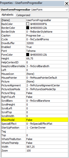
EXCEL has a built in mechanism to store and retrieve userform controls values. This is done through a property called "ControlSource". It is present on the properties of a control. See below for the CheckBox control:
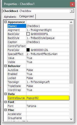
This ControlSource property can be made to point to a cell. This will retain the value also when the workbook is stored. As an example I have linked one control box to cell B2 in Sheet "PopUp" and the other to B3:
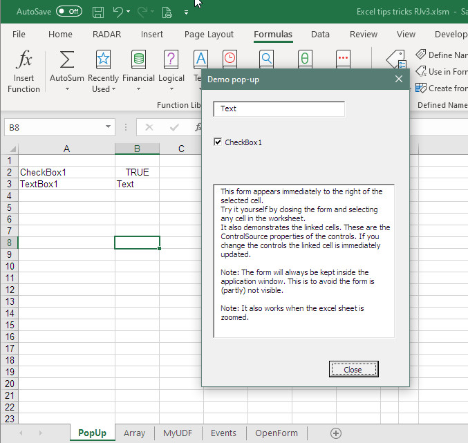
In the above example the values are stored on the fly on the sheet. As soon as you change a value on the form it is stored in the sheet. No additional code is needed! When the workbook is saved the values are also automatically saved. When the userform is activated again it uses the stored values in the linked cells as the initial startup value. You can make the sheet hidden and give it a proper name, like 'Settings'.
Position of (pop-up) window on the screen and worksheet
When you use a form in your code that pops-up you may want to position it more precisely. Excel offers a few options in the properties of the form during design:
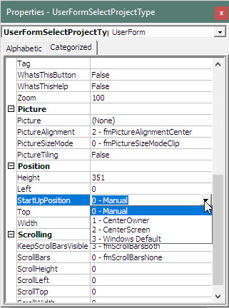
- Manual : Userform will retain position between subsequent hides and shows. Initially userform will be positioned top-left of the screen. If the user changes position of the Userform by dragging and the window is 'closed' with the Userform.Hide method then on the next Userform.Show the Userform comes back on its previous position. If you close the window with the X this unloads the userform and the position will revert to top left again. Note that this can be outside the excel window if this is not maximized.
- CenterOwner : Userform appears center vertical and horizontal of the excel application window. If excel window is maximized this is the same as CenterScreen
- CenterScreen : Userform appears center vertical and horizontal of the screen. Note that this can be out of the excel window if the excel window is not maximized.
- WindowsDefault : Userform appears top-right of the screen. Note that this can be out of the excel window if the excel window is not maximized.
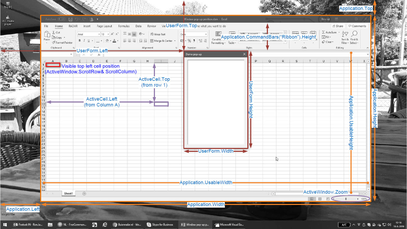
In mode 'Manual'when you want more control or dynamically change the position you can do this in the VBA code. There are a couple of Application, Userform and ActiveCell properties that are (can be) involved. This is shown in the picture below:
From the above picture you would expect that the minimum value for .top and .left are 0. But in fact, in a multi monitor set-up, these values can go below 0 and beyond the right side of the screen. This all depends on the position of the monitor in the windows configuration. The reference for the .top and .left values is normally monitor #1. This was a setup with a laptop and 2 connected monitors. Monitor #1 was the laptop screen:
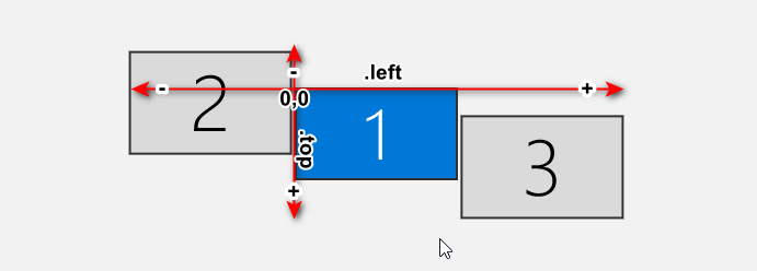
But I also had a situation where not monitor #1 was the reference but monitor #2 appeared to be the reference. This occured after I closed the laptop screen. In the picture below both monitor #1 and #2 are external monitors. So windows renumbered the monitors when I closed the laptop:
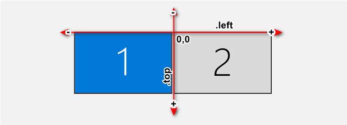
With the excel application moved to monitor #2 you would get negative values for the .left and possibly also for the .top. With all this in mind I use the following code in a module to position a userform right of a selected cell (as shown in the above picture):
Note that this procedure uses ByRef for the parameters, normally this is ByVal. ByRef allows the procedure to modify the parameters. In this case set the window .left and .top properties. This procedure is called from the Userform.Initialize event:
Private Sub UserForm_Initialize()
	WindowPosRightOfSelection UserForm, ActiveCell
End SubNote: If you would execute this code directly from the userform then the 'w' should be replaced with 'Userform' or 'Me' and the 'c' should be replaced with 'ActiveCell. For instance var>w.Top becomes Me.Top and c.Left becomes ActiveCell.Left
The main part of the routine is:
	w.Top = Application.Top + c.Top * ZoomLevel + CommandBars("Ribbon").Height - (w.Height / 2)
	w.Left = Application.Left + (c.Left + c.Width) * ZoomLevel + (w.Width / 4)
This code will override the default startup position that was set in the form. The ActiveCell properties are affected by the excel window zoom level (in the bottom right corner). To calculate the position correctly you have to multiply the ActiveCell.Left and ActiveCell.Top values with the zoom level factor. I used the ribbon height property to account for a (un)collapsed ribbon.
- Hiding a userform with
Userform.Hidekeeps it in the background. It means that values on the form will be saved during the session. - Clicking on the X of the userform 'unloads' it. This means that values on the form are not saved. The form is re-initialized again (event:
UserForm_Initialize()) when it is shown. - When the userform is made visible this triggers the activate event
UserForm_Activate() - The ActiveCell.Top and ActiveCell.Left properties are the distances respectively from Row 1 and Column A. So not from the left / top of the excel window grid! This means that when the excel window is scrolled and row 1 and/or column A is not visible you get a too high value for the ActiveCell.Top and ActiveCell.Left properties
- It is good practice to check if userform is not positioned off screen or off excel window. If the userform is positioned off screen you cannot close it and this may block code execution.
- The Application.UsableHeight and Application.UsableWidth properties give roughly a size that is a little bit bigger than the cell grid.
Using arrays to speed up read and write to worksheet cells
Reading from and writing to worksheet cells takes up relatively much of the processing time of code. A faster way to do this is to use an array to store, modify and restore the cells. Increase in speed can easily be a factor 100x. Steps to follow if to use an array
- Define an array without dimension eg ArrRange() as Variant. USe type variant to handle all types of values (strings, integers, dates etc) in a cell
- Define the range / area you want to work on.
- Re-define the array using the range column and row values.
- Read the sheet values into the array.
- <code that manipulates the array values>"
- Write the array back to the worksheet
In excel basic this could be something like:
Sub DemoWriteCells()
Dim ArrRange() As Variant
Dim StartRange As String
Dim EndRange As String
Dim rDim As Integer
Dim cDim As Integer
Dim r As Integer
Dim c As Integer
Dim sTime As Date
Dim fTime As Date

' define the range to work with
TopLeftCell = "B5"
BottomRightCell = "BZ100"

' First directly write to cells on the worksheet
sTime = Now()
For r = Range(TopLeftCell).Row To Range(BottomRightCell).Row
	For c = Range(TopLeftCell).Column To Range(BottomRightCell).Column
		Worksheets("PopUp").Cells(r, c) = "w"
	Next c
Next r
fTime = Now() - sTime
MsgBox "Execution time direct write to cells = " + CStr(fTime), vbInformation

' Use array to read and write cells on worksheet
rDim = Range(BottomRightCell).Row - Range(TopLeftCell).Row
cDim = Range(BottomRightCell).Column - Range(TopLeftCell).Column
ReDim ArrRange(rDim, cDim)
ArrRange = Range(TopLeftCell + ":" + BottomRightCell).Value

sTime = Now()
For r = 1 To Range(BottomRightCell).Row - Range(TopLeftCell).Row + 1
	For c = 1 To Range(BottomRightCell).Column - Range(TopLeftCell).Column + 1
		ArrRange(r, c) = "A"
	Next c
Next r
Range(TopLeftCell + ":" + BottomRightCell).Value = ArrRange
fTime = Now() - sTime
MsgBox "Execution time using array = " + CStr(fTime), vbInformation

End Sub
Note, the .value property of the cell is used in the above example to read and write back the data. Excel stores values and formulas of a cell separately from each other. The .formula property holds the formula and the .value property will hold the result. Writing to a cell using the .value property looses the formula if there was one. If you are working with an area that (also) holds formulas then consider using .formula to read and write the data.
Adding a menu to the ribbon.
To make your excel code more user friendly and professional you can add command buttons to the built in excel ribbon.
- You can define yourself where the new menu should be positioned in the ribbon.
- You can give the menu and the buttons a short name. This name is visible on the ribbon.
- You can define an icon from the standard set. For a list of names search for 'msoImages' on the web.
- Or you add a new icon to CustomUI and use that.
- You can add tooltip text to your buttons. This will appear if the user hovers over the button with the mouse.
- You can enable or disable a button. A disabled button will be grayed out.
The following steps are needed to add a menu to the ribbon:
- If not already done, download and install the CustomUI utility.
- From CustomUI open an xlsm file and add xml code for the ribbon.
- Save the xml code to the excel
- Open the xlsm in Excel. You will now see the added menu
- Add code to a module in the xlsm to handle the events triggered by the buttons.
Here is an example of xml code for a menu in the ribbon:
	<ribbon>
		<tabs>
			<tab id="customTab" label="RADAR" insertAfterMso="TabHome"
				<group id="customGroup1" label="Tools"
					<button id="customButtonIMP"
						label="Import workload"
						size="large"
						screentip="Imports the capacity and planned workload from the VIRES export file."
						supertip="Refreshes the data in sheet WorkloadImport."
						onAction="cMenuImportWorkload"
						enabled = "true"
						imageMso="RecordsAddFromOutlook" />
					<button id="customButtonOPL"
						label="OPL list"
						size="large"
						screentip="Update the prospect/sales projects list from an OPL file on the server"
						supertip="Reads the OPL file and updates the project data."
						onAction="cMenuUpdateOPLRadar"
						enabled = "false"
						imageMso="CacheListData" />
					<button id="customButtonSORT"
						label="Sort OPL"
						size="large"
						screentip="Sorts the OPL list."
						supertip="1) Area[A-Z] 2) Scoring Chance[Planned,High,Medium] 3) Start Eng Req[Old-New]"
						onAction="cMenuSortOPLList"
						enabled = "true"
						imageMso="SortCustomExcel" />
					<button id="customButtonHLP"
						label="Manual"
						size="large"
						screentip="Open the user manual of the Radar excel file."
						supertip="Opens the pdf version of the user manual stored in smarteam under document number A_DOC384967."
						onAction="cMenuHelp"
						imageMso="FunctionsLogicalInsertGallery" />
				</group>
			</tab>
		</tabs>
	</ribbon>
</customUI>
And here is the event handling code for the above ribbon:
' button [Import]
' Callback for customButtonRes onAction
'
Sub cMenuImportWorkload(control As Variant)
    ' insert code here to execute
    MsgBox "Menu button 'import workload' pressed", vbInformation
End Sub
'
' button [Update OPL]
' Callback for customButtonOPL onAction
'
Sub cMenuUpdateOPLRadar(control As Variant)
    ' insert code here to execute
    MsgBox "Menu button 'update opl radar' pressed", vbInformation
End Sub
'
' button [Sort OPL]
' Callback for customButtonSORT onAction
'
Sub cMenuSortOPLList(control As Variant)
    ' insert code here to execute
    MsgBox "Menu button 'sort OPL list' pressed", vbInformation
End Sub
'
' button [Manual]
' Callback for customButtonHLP onAction
'
Sub cMenuHelp(control As Variant)
    On Error Resume Next
    ActiveWorkbook.FollowHyperlink Address:="http://members.home.nl/rjut/EXCEL/CustomUI sample of ribbon.jpg"
    On Error GoTo 0
End Sub
Download the excel file for the code. Check out module4_CustomMenu and the excel ribbon.
Making your own custom functions.
EXCEL has many useful built in functions that you can use in your spreadsheet. Sometimes you miss a function that is not available. I needed for instance a function to split a separated string into different individual elements, each in their own cell. Splitting a string such as "one, two, three". Three words separated by a comma. If you want each element in a different cell then of course you can do this with the standard built in 'text to columns function':
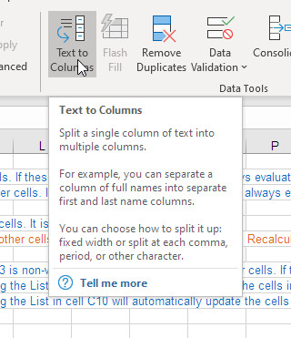
... but this is static and I wanted a dynamic split. Of course you can also use the standard excel functions but this is cumbersome. First you need to find the location of the commas, then you extract each element into a different cell. Excel VBA offers a very simple built in function called split() for this. You can make a so-called User Defined Function (UDF) that can be used in the excel spreadsheet and that uses the VBA split function to do the work.
There are a couple of important things to remember with UDF's:
- An UDF must reside in a module.
- An UDF must be a function that returns a single result.
- An UDF function can reference any other cell in the workbook but cannot manipulate other cells in the spreadsheet or workbook. Excel will not allow this.
- An UDF is by default a so-called 'non volatile' function. This means that EXCEL will only (re)calculate the result if it directly depends on another cell in the workbook. For instance
=MyUDF(A3)depends on cell A3 so is always recalculated if cell A3 changes. To make sure cells with your UDF are recalculated properly you can either force the function to be volatile or use another cell reference as a parameter of the function. There is actually a third method and that is to manually force recalculation of the complete workbook by pressing Ctrl-Alt-F9. If you force the function to be volatile then excel will always recalculate, even if the parameter values of the function did not change. If you have many (thousands) of cells with a volatile function then EXCEL will always recalculate all these thousand cells if you change something to the worksheet. You may start noticing a delay after changing a cell. If you use a cell ref as a parameter then EXCEL will only recalculate the UDF when the cell referenced changes.
If you want to know more about UDF's in excel check out this excellent website. See below for an example of a UDF function:
Function MyUDF3(SepList As String, SepChar As String, ElPos As Integer)
Dim SepArr() As String
Dim i As Integer
	' split the string into a zero based array
	SepArr = Split(SepList, SepChar)
	' return the requested element from the array
	MyUDF3 = SepArr(ElPos - 1)
End Function
This function returns the ElPos'th element from a list string SepList were elements are separated by SepChar. It could be used in an excel sheet cell as =MyUDF3(C9,";",2) which will return "b" into the cell when cell C9 holds "a;b;c;d;e". When used like this EXCEL will (re)calculate the result if cell C9 is changed
If your UDF does not reference other cells and you want to force the function to be volatile then:
Function MyUDF() As Double
	' Good practice to call this on the first line.
	Application.Volatile
	MyUDF = Now()
End Function
This function simply returns the time. Of course this is already a built in EXCEL function
There are a couple of UDF's in this module:
- MyUDF1 adds the vaule of 2 cells and can be set to volatile or non-volatile with a parameter. It demonstrates that it is always recalculated, volatile of non-volatile.
- MyUDF2 simply returns the time and can also be set to volatile or non-volatile with a parameter. It demonstrates that it is only recalculated when it is volatile, parameter is TRUE.
- MyUDF3 is the list separator function. It references another cell for the SepList parameter. It demonstrates that it is recalculated when the referenced SepList cell changes. It is more elegant when you call this function in the sheet with
=MyUDF3($C9;",";COLUMN(D9)-COLUMN($C9)). This way the parameters change to the next index when you copy the cell to other cells. - MyUDF4 is another list separator function. It uses an indirect reference to another cell for the SepList parameter. It uses this indirect ref to determine the number of cells between the calling cell and the cell with the list. Therefore it does not need the ElPos parameter. But since the cell reference is indirect it is not recalculated automatically ... unless you change the way you call it. In the excel sheet I used
=MyUDF4("C"&ROW($C14);";")to call the UDF. By using $C14 as a reference the cell is re-calculated when the list in cell C14 changes. If you copy the formula to other rows then it is also correctly changed by excell. Or of course you can add the lineApplication.Volatileto your code to make sure it is always recalculated. Then you could call the function simply by=MyUDF4("C13";","). - MyUDF5 is the same as MYUDF4 but forced volatile.
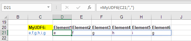
- MyUDF6 is by far the most efficient and user friendly version. This only works with the new excel array formulas and spill functionality available from 2019/2020 in Excel Office 365 v16. This function has only one line of code!. It simply directly returns the result of the
split()function. This is an array. In previous excel version this would result in a single value entered in the column where the formula is entered. In the latest versions excel fills in all returned array values into adjacent cells. This is called spilling. For this to work the cells next to the formula have to be empty. If not a SPILL error is shown in the formula cell. Note that the formula is entered only in one cell. Note also that if you change the number of items in the list the spill range will automatically be sized to the number of elements, cool! If you select the cell with the formula the spill range will be marked with a blue border:
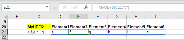
If you select another cell of the spill range the formula will be shown in gray.
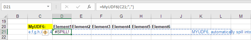
If the entire spill range is not empty then you get the SPILL error in the formula cell:
For splitting a list I prefer to use =MyUDF6(C21;",") because I have the latest EXCEL version. For older versions of EXCEL I would use the =MyUDF4("C"&ROW($C14);";"). It is only recalculated when needed and can be easily copied to other columns and rows.
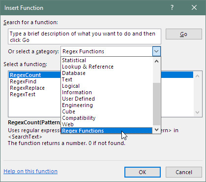
One very nice possibility is that you can define your own help text for a user defined function. This help text appears in the excel function selector. Also you can put your UDF's in their own category. To do this you have to run the following code for each function you want. You have to run this code only once. Therefore I placed it in the ThisWorkbook module in the Worksheet_Open() event:
Application.MacroOptions _
	Macro:="MyUDF3", _
	Description:="Returns the n-th element from an one dimensional array", _
	Category:="User Defined", _
	ArgumentDescriptions:=Array("String with text reference to a cell with the array list with the separated elements.", "The separation character used in the list.")
The result is shown in the function input pop-up form:
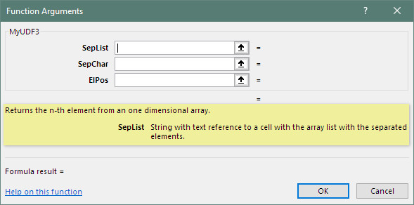
In the above example the MyUDFx user function definitions are added to the (excel predefined) category 'User Defined'. You can also create your own new category. As an example:
The difference between HIDE and UNLOAD of a form.
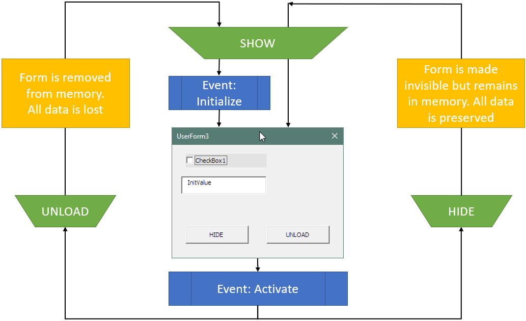
An excel form is made visible with the command UserFormX.Show in the vba code. It can be made invisible with the command UserFormX.Hide or with the command Unload UserFormX. They both seem to do the same thing, but there is a difference. I like to think of it this way: With Hide the form is simply made invisible but is still active in the background. With Unload the form is removed from memory completely. The difference can (does not have to be) be visible when you re-open the form using the command UserFormX.Show again. When the form was closed with UserFormX.Hide the form is opened at the same position it was when it was closed and the values of the controls are kept. When the form was closed with Unload UserFormX the it is re-initialized again. All properties are set as defined during design time. The event 'UserFormX_Initialize' is triggered when the form is opened for the first time or after an unload. The event 'UserFormX_Activate' is triggered when a form is opened after hide and also after unload. When the 'UserFormX_Initialize' event is triggered the form is being built but not yet shown to the user. When the event 'UserFormX_Activate' is triggered then the form has just been opened and is shown to the user. This is why the window position manipulation code in the above example is inside the 'UserFormX_Initialize' event. In the picture below I have tried to illustrate this graphically:
The difference between unload and hide is normally not so relevant. You can place 'the code to execute' when form is started in the 'UserFormX_Activate' event. I ran into some situations where this difference became important:
- When you want to manipulate the position of the form programmatically.
You want this code to execute before the form is shown i.e. in the UserFormX_Initialize event. This also means that the form must be closed withUnloadotherwise the UserFormX_Initialize event is not triggered afterUserformX.Show - When you use a value of a form control in your VBA code.
When a form is UNLOADed and you check (egResult = CheckBox1.Value) or change (e.g.CheckBox1 = False) the value of a CheckBox control in your code, then this triggers also the UserForm_Initialize event of the form where the controls is on. In this case you want to close the form with hide. See section Progressbar for an example.
Download the excel file to try it yourself. Check out sheet 'OpenForm' and UserForm3.
Events triggered by the form controls.
The controls on a userform can trigger a myriad of events. The events can be triggered by the user or by other VBA code. All controls seem to have events that can be triggered but these are not the same for all controls. A commonly used event is the Click() event which is generated when the user clicks on the button with the mouse or presses the ENTER key when the command button has the focus (dotted line visible on the button). Below is a summary of some commonly used events
| Event: | Parameters: | Explanation: |
|---|---|---|
| ContolX_Change() | - | This event is triggered when the user has changed the value of the control or the value is changed programmatically in VBA code. |
| ContolX_Click() | - | This event is triggered when the user has clicked on the control or the control is assigned a value in VBA code. |
| ContolX_MouseDown() ContolX_MouseUp() |
Button X Y |
This event is triggered when the user has clicked on the control. The X and Y in points give a relative point where the user clicked. TopLeft is 0,0. X is to the right and Y is down. Button is the mouse key that was pressed. Left=1, Right=2, DblClick=4 |
| ContolX_KeyDown() ContolX_KeyUp() |
KeyCode | This event is triggered when the user has pressed or released a key. The KeyCode holds the value of the key pressed/released. Click here for a list of KeyCodes |
ContolX_KeyPress() | KeyAscii | This event is triggered when the user has pressed a key. The KeyAscii holds the character of the key or key pressed. The difference between a KeyCode and a KeyAscii is that a KeyCode represents 1 key on the keyboard. A KeyAscii is an actual visible character that can be read. For instance shift key has KeyCode=16 dec, Letter A has KeyCode=65 dec. Typing Shift+A will result in 2 key codes, one for the shift key and one for the A key but only 1 ASCII code 65 Click here for a ASCII character table. |
More than one event can be (and usually is) triggered by a single action. Below are some examples of what events are triggered by what action on a control:
| Controls: | Action: | Events triggered in order: | Explanation |
|---|---|---|---|
| CommandButton | Mouse click on button when control has focus |
|
Using Click() to detect button pressed is most commonly used. |
| CommandButton | ENTER key pressed when control has focus |
|
Using Click() to detect button pressed is most commonly used. |
| Label | Mouse click on the label |
|
|
| Image | Mouse click on the image |
|
The X & Y values can be used to do a certain action depending where in the image the user has clicked |
| CheckBox | Mouse click on the checkbox |
|
|
| CheckBox | Change value programmatically e.g. CheckBox1.Value = True |
|
|
| OptionButton | Mouse click on a unchecked option button X that is part of a group. |
|
The first EXIT() event is of another option button in the same group After the mouse click you get 2 change events, one for the previous button and one for the current button. |
| TextBox | Clicking in a text box and editing the contents followed by pressing ENTER key. |
|
The MouseDown/Up events appear after clicking in the text box. For every key pressed you get a KeyDown/Up event For every printable/visible character you get a KeyAscii event. For every modification to the contents you get a change event. The last KeyDown is for the ENTER key. |
| General | When control X looses focus due to pressing TAB key or clicking another control. |
|
|
| General | When control X receives focus due to pressing TAB key or clicking on control X. |
|
There are 2 properties that influence the events that can be triggered by a controls. These are "Enabled" and "Locked". Both of these can be set to True or False.
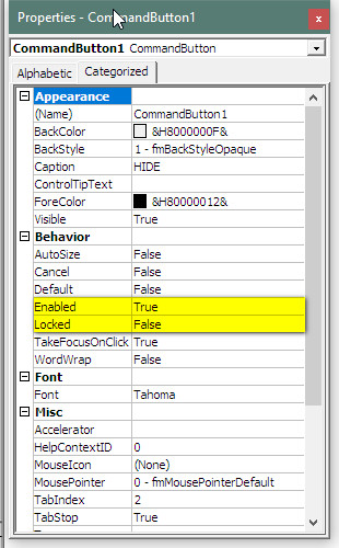
The Enabled property set to False greys out the control on the UserForm. In this state it does not generate events anymore when clicked. It also cannot get the focus. So it seems completely dead.
With the locked property set to True the controls is shown as normal on the form. The user cannot change/modify it. It can still receive focus. It will still generate some events.
To demonstrate all this I have made a UserForm2 that lists the events that the user can trigger on various controls.
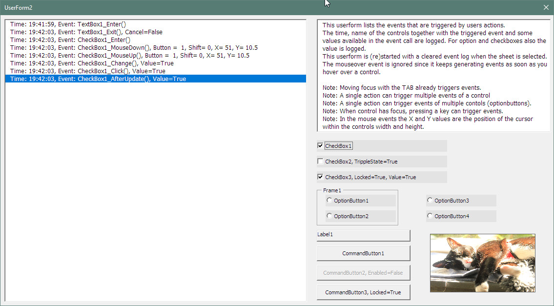
Download the excel file to try it yourself. Check out sheet 'Events' and UserForm2.
Regular expressions with user defined functions.
The built in search/replace function in excel is very useful and flexible. It can find text in cells or formulas and also certain formatting of a cell. The user interface allows for some special characters to look for specific text. I believe the options are:
- * to find any combination of characters. For instance 'the*re' would find a cell containing 'there' but also 'they were'.
- ? to find any single character. For instance 'the?e' would find a cell containing 'there' but also 'theme' but not 'they were'.
- ~ To escape a * or ?. For instance you would use ~* to search for a single *
- ALT+nnnn You can type in a 4 digit char code by holding the ALT key while typing the 4 numbers on the num keypad.
Editors such as Notepad++ have a more powerful find and replace. Notepad++ uses a text find/replace syntax that is known as 'regular expressions'. This is a rather cryptic yet powerful syntax that enables more complex search and replace actions. The syntax with regular expressions is not fully standardized. Every implementation seems to differ a little from the other. However, many frequently used options are common.
Microsoft Office has a regular expression engine already built in that can be made available for the excel user through User Defined functions. I have made a couple of user defined functions so that you can get familiar with the (microsoft office) syntax of the regular expressions.
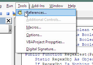
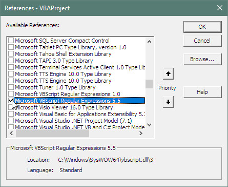
The regular expression engine is part of a library that is not by default included in the excel workbook. You have to include it yourself. This can be done in the Visual Basic editor through the tools menu:
Select the 'Microsoft VBSript regular expressions 5.5' library. Make sure not to include the old 1.0 version.
In the workbook I have added a sheet 'Regex' and a module 'Module2_RegularExpressions'. To keep the user defined functions as compact as possible I have created 4 user defined functions to cover 4 different scenarios (Test, Find, Count and Replace). All 4 functions are almost identical. Below is the one for RegexTest.
Module1_RegularExpression:

Const ParGlobal As Boolean = False     ' FALSE=Single match, TRUE=Find all matches
Const ParIgnoreCase As Boolean = False ' FALSE=case sensitive, TRUE= a equals A
Const ParMultiLine As Boolean = False  ' FALSE=Anchor $ is end of line, TRUE=anchor $ is end of file. For text string use in this excel this should be FALSE.
Dim RegexObj As New VBScript_RegExp_55.RegExp ' Creates a static RegExp object used by the Regex routines in this module

Public Function RegexTest(Pattern As Range, SearchText As Range) As Boolean
	With RegexObj
		.Global = ParGlobal
		.Pattern = Pattern
		.IgnoreCase = ParIgnoreCase
		.MultiLine = ParMultiLine
	End With
	RegexTest = RegexObj.test(SearchText)
End Function
The first four lines define module wide constants that are used in each of the 4 user defined regex functions.
The fith line defines an regular expression object that is used in the module. This object is created onces. This improves execution time. With a 'Dim RegexObj' in every function it took about 3 seconds to process 2000 cells. With the module level 'RegexObj' it takes about 1 second. The with statement set the parameters and the search pattern. Finally a method 'test' is invoked with the SearchText
Note: For some reason the RegexReplace did not function with the module level object. This function creates its own static object. If a reader can tell me why this is happening, please drop me a mail!.
The sheet is built up as follows:
- In column A there is a list of 2000+ text entries. This is the SearchText
- Test: In column B the user defined function used is RegexTest(Pattern, SearchText). The Pattern is entered in the header of the column. The SearchText is directly left of the formula in column A. The result of the formula is shown in the cell in column B. FALSE when the Pattern is not found in SearchText, TRUE if it is found.
- Count: In column C is RegexCount(Pattern, SearchText). The Pattern is entered in the header of the column. The SearchText is directly left of the formula in column A. The result of the formula is shown in the cell in column C. 0 if not found, 1 if found once, 2 if found twice etc...
- Find: In column D is RegexFind(Pattern, SearchText). The Pattern is entered in the header of the column. The SearchText is directly left of the formula in column A. The result of the formula is shown in the cell in column D. #N/A if not found, The found text if found once or #VALUE if found more than once.
- Replace: In column E is RegexReplace(Pattern, SearchText, ReplaceText). The Pattern is entered in the header of column E. The SearchText is directly left of the formula in column A. The ReplaceText is in the header of column F. The result of the formula is shown in the cell in column E. The original SearchText> if not found, The replaced text if found.
- In column H is a quick reference to the most used regular expression syntax of Microsoft office. The full list is available on the Microsoft website.
As an example I have made a regular expression pattern to replace a song file name with another file name. The search/replace patterns replace "The Artist" with "Artist, The".
The search string used for this is: 'Singles\\(The)\s(.+)\s-\s'
This looks rather cryptic but if you brake it down into smaller pieces and check with the quick reference it all makes sense.
- 'Singles' text simply searches/matches the text 'Singles'. Keep in mind that the search is case sensitive.
- '\\' refers to the backslash character following the text Singles.
- '(The)' captures the word 'The' and stores in group 1. Group 1 because it is the first time a group is defined.
- '\s' represents a space character following 'The'
- '(.+)' captures the text up to ' - ' and stores in group 2
- '\s-\s' is the dash separator between artist and title including the spaces
A typical search result for input text "Singles\The Rolling Stones - Emotional Rescue.Mp3" would be "Singles\The Rolling Stones - " where 'The' is captures in group 1 and 'Rolling Stones' in group 2.
The replace string used for this is: 'Singles\\$2, $1 - '
This breaks down to:
- 'Singles' literal text 'Singles'
- '\\' to insert the \ character
- '$2' inserts group 2
- ', ' inserts a comma and a space
- '$1' inserts the first group
- ' - ' finally the artist and title separation is added again.
The replacement result is "Singles\Rolling Stones. The - "
The function returns a string where the match result in the SearchText is replaced. So "Singles\The Rolling Stones - " is replaced with "Singles\Rolling Stones. The - "
This is something that cannot be achieved with the built in find/replace of excel.
Download the excel file to try it yourself. Check out sheet 'Regex' and Module1_RegularExpression.
Reading user applied filter settings
In VBA you can programmatically read and manipulate the filters of a table. Let use this table as an example:
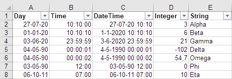
You can read the filter settings for example with the following code or something similar:
	Dim cr1 As Variant
	Dim cr2 As Variant
	Dim fon As Boolean
	Dim FilterText As Filter

	Set FilterText = ActiveSheet.AutoFilter.Filters(5)
	fon = FilterText.On
	If fon Then
		ope = FilterText.Operator
		cr1 = FilterText.Criteria1
		cr2 = FilterText.Criteria1
	End If
The 5 means the 5th column of the filter table. The fon is only true if column 5 is being filtered. If another column is filtered but 5 is not then it will be false. The cr1 and cr2 are defined as variant because these values are not always strings as you will see below. The first thing you need to do if the filter setting is actually active. If it is not active an attempt to read the Operator and Criteria1 and Criteria2 will result in a runtime error.
I found out the hard way that this approach does not work for multi level selection filter that is used for dates:
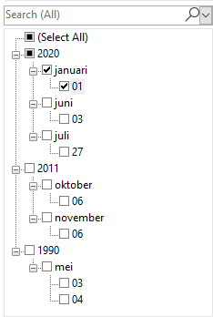
Even when filtering is active on a date column, an attempt to read Criteria1 and Criteria2 will result in a runtime error. Do not know if this is intended or a bug in EXCEL. You can happily read the fon and Operator. Strange thing is that you can set the multilevel filter criteria programmatically but even then you cannot read them back! You can use for instance the following to set a filter on a multi level date column:
	' filter date column
	' criteria2 array(depth, "m/d/yyyy hh:mm:ss")
	' depth sets filter depth, 0=year, 1=month, 2=day
	ActiveSheet.Range("A1:E8").AutoFilter Field:=1, Operator:=xlFilterValues, Criteria2:=Array(2, "5/3/1990")
Note that the date format has to be in American
style mm/dd/yyyy. For multi level filtering Criteria1 is not used. Criteria2 is an array consisting of 1 or more pairs of number followed by a date. The number indicates the level/branch on which the filtering is applied. A 0 for years, a 1 for months and a 2 for days. With a 0 and a given date all dates in that year will be checked and visible after filter is applied.
However, the filter settings are stored in the EXCEL workbook. This can be proven by closing the workbook and opening again. On re-opening the filter will show the setting before it was saved. The settings are stored in the sheetX.xml file inside the ZIPped Excel xlsm file. X being the sheet number. In this workbook it is sheet7. In the xml it is stored as:
<autoFilter ref="A1:E8" xr:uid="{8CFF16D5-699F-4856-ADBB-D7A55000C510}"><filterColumn colId="0"><filters><dateGroupItem year="2020" month="5" dateTimeGrouping="month"/><dateGroupItem year="1990" month="5" day="3" dateTimeGrouping="day"/></filters></filterColumn></autoFilter>
| User selection | Table result | Operator | Criteria1 | Criteria2 | Remark |
|---|---|---|---|---|---|
1 value selected |
 |
0 | "=Delta" | 'undefined' | There is no enumeration defined for 0. This works only for a single level selection list as shown, NOT for multilevel date selection! |
2 values selected |
 |
2 = xlOr | "=-102" | "=21" | This works only for a single level selection list as shown, NOT for multilevel date selection! |
3 values selected |
 |
7 = xlFilterValues | {"=00:00:01", "=07:00", "=23:59:59"} | 'undefined' | Criteria1 is 1d array with 3 values. This works only for a single level selection list as shown, NOT for multilevel date selection! |
Between start and end values |
 |
1 = xlAnd | "=1‑1‑2020" ">=43831" | "=1‑1‑2021" "<="44197" | Custom filter between 1-1-2020 AND 1-1-2021. Criteria1 and Criteria2 hold the date in human readable format or as the equivalent number. Not sure why it sometimes displays one or the other. |
Date filter eg 'Year To Date' |
 |
11 = xlDynamic | 16 | 'undefined' | Criteria1 holds specific date filter, see microsoft.com" for a full list of all possible enumerations. |
| Multilevel selection. ActiveWindow.AutoFilterDateGrouping = TRUE  |
 |
7 = xlFilterValues | 'undefined' | 'undefined' | Both Criteria1 and Criteria2 have no value. An attempt to read Criteria2 in VBA code will actually result in an error. No way to retrieve the filter settings through Criteria2. Even if this filtering was not set by the user but was set using VBA code then you would still not be able to read the settings back through Criteria2. |
| Single level date selection. ActiveWindow.AutoFilterDateGrouping = FALSE  |
|
2 = xlOr | "=03‑05‑90" | "=03‑05‑20" | Same as other type filtering with 2 values. Compare above filtering on 2 numbers. Criteria1 and Criteria2 date format is same as selected for the date column in the table. |
Working with the UsedRange
The Sheet1.UsedRange in Excel can be handy if you want to work in VBA will all cells, rows or columns of the sheet. It is the smallest rectangle range that includes all used cells on a sheet.
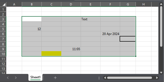
In the above screenshot the UsedRange spans from cell B3 to G10. So the address of the UsedRange (Sheet1.UsedRange.Address) is "$B$3:$G$10". The UsedRange is automatically updated by Excel when the range of used cells changes. Also when the sheet is modified using VBA code. There are a few things to notice about the UsedRange:
- it includes cells with any type of value, number/text/date etc
- it includes cells with a formula, even if formula result is empty
- it may not start at first row/column of the sheet
- it can included empty cells/rows/columns
- it include cells with only formatting and no value
- it includes cells with a note or comment
It seems that any kind of formatting classifies the cell 'used'. Such as horizontal/vertical alignment, text font type/size/color/underline/bold/italic, cell fill color, cells border. To be more precise, a cell is classified as 'used' if the formatting of the individual cell differs from the formatting to all the cells in the sheet. This is done by pressing Ctrl-A or by clicking the rectangle in the top left corner of the sheet. This selects all cells on the sheet. Any formatting applied to all the cells does not affect the UsedRange.
There are also some settings that do not affect the UsedRange, i.e. does not classify a cell 'used'. This is what I found so far:
- conditional formatting of the cell
- data validation on the cell
The UsedRange on a new and empty sheet is not 'nill' as you may expect but is "$A$1".
You can check yourself the bottom right corner of the UsedRange on a sheet by pressing Ctrl-End. This moves the selection to the last row and column of the UsedRange. Sometimes this is an empty cell and it may not immediately be clear why this cell is included in the UsedRange. To correct this you select this row and all the rows up to just below your data. Then choose 'Delete-Rows' in the menu. Do not use 'Clear'. Do the same with the columns. This should reset your UsedRange again. If not press the 'Save' button once. In VBA you use the command Sheet1.UsedRange.Calculate. This is needed to refresh the UsedRange. As far as I know there is no way to goto the top-left corner of the used range with a shortcut key. You could type Sheet1.UsedRange.Select in the immediate window and check the sheet. The UsedRange is now highlighted/selected.
To retrieve the nr of rows in VBA of the UsedRange you can use Sheet1.UsedRange.Rows.Count, or Sheet1.UsedRange.Rows.CountLarge for a large nr of rows. For the nr of columns you can use Sheet1.UsedRange.Columns.Count, or Sheet1.UsedRange.Columns.CountLarge.
To retrieve the number of the first row or first col use Sheet1.UsedRange.Rows(1).Row or Sheet1.UsedRange.Columns(1).Column
You can use the count of rows to loop through each row of the UsedRange:
Sub UsedRangeLoopRowNrs()
	Dim i As Integer
	Dim rRng As Range
	Debug.Print "Index", "Row nr"
	For i = 1 To Sheet1.UsedRange.Rows.Count
		Set rRng = Sheet1.UsedRange.Rows(i)
        Debug.Print i, rRng.Row     ' prints the index nr and the actual row nr in the immediate window
	Next i
End Sub
This would give the following output from the example above:
Index         Row nr
 1             3
 2             4
 3             5
 4             6
 5             7
 6             8
 7             9
 8             10
Or though the columns:
Sub UsedRangeLoopColumnNrs()
	Dim i As Integer
	Dim cRng As Range
	Debug.Print "Index", "Column nr"
	For i = 1 To Sheet1.UsedRange.Columns.Count
		Set cRng = Sheet1.UsedRange.Columns(i)
		Debug.Print i, cRng.Column     ' prints the index nr and the actual column nr
	Next i
End Sub
This would give the following output:
Index         Column nr
1             2
2             3
3             4
4             5
5             6
6             7
Alternatively, you can use a 'for each loop' to itterate through all the used rows of a sheet:
Sub UsedRangeLoopRows()
	Dim uRng As Range
	Dim cRng As Range
	For Each uRng In Sheet1.UsedRange.Rows
		Debug.Print uRng.Row        ' this print the row nr
		Set cRng = uRng.Columns(1)  ' this is the first cell in the row
	Next uRng
End Sub
To go through all the used cells also a 'for each loop' can be used:
Sub UsedRangeLoopCells()
	Dim cRng As Range
	For Each cRng In Sheet1.UsedRange.Cells
		Debug.Print cRng.Address, cRng.Row, cRng.Column  ' prints the address of the cell
	Next cRng
End Sub
Userform show/goto row & col number
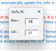
In Excel, like most people, I always work with number for rows and letters for columns. The so-called A1 style notation. In VBA I sometimes refer to sheet cells using Range.Cells(11,12), so using numbers for the column. To test and verify code it can be useful to know in Excel what the column nr is. You can set the R1C1 ref style in the Excel option to show column nrs in the sheets, but you have to switch it back later. For just one or a few column nrs this is cumbersome. Therefore I made a small UserForm that shows the row and column nr in an input box on a userform. Linked to a shortcut key it can quickly show you the info. In the attached excel file it is linked to Ctrl-r. Moreover, it doubles as a GoTo Row & Col nr. If you change the row and/or col nr followed by the enter key it will select that cell and exit the form. So you can also use it to find out what column letter column nr 123 has, for instance. The userform always appears in the middle of the screen. Pressing escape will also close it but not do a jump. There is no validation on user input so if you give a non-number then the code will break.
You can set the Excel option for R1C1 style notation with VBA in the IDE immediate window. If you type Application.ReferenceStyle = xlR1C1 your excel window will now show column numbers. Of course, also the formulas will be shown in R1C1 style. To go back you type Application.ReferenceStyle = xlA1 and it will switch back.
Calling sub and functions
The section is about calling subs and functions from worksheets and modules. The principle is the same for subs and functions, so for now will only mention subs. What is allowed and possible depends on how the sub is defined. In calling subs a userform or class module follows the same rules as a module.
- When a sub is defined with the PRIVATE keyword, it can only be called from the same worksheet or module where it is defined
- When the sub is declared with the PUBLIC keyword it can be called from other worksheets or modules
- When calling a private sub you just use the name (so always on the same module or worksheet)
- When calling a public sub on the same module or worksheet you just use the name, so no difference with a PRIVATE sub
- When calling a public sub defined on a module from another worksheet or module you just use the name
- When calling a public sub defined on a worksheet from another worksheet or module you prefix the name of the worksheet where the sub is defined
- events on worksheet are by default PRIVATE but can be made PUBLIC. In that case these can also be called from other worksheets or modules when you prefix the name of the worksheet
- when more modules have public subs with the same name you have to prefix a worksheet call with the module name. A call from a module will by default run the sub on the same module.
In the table below a more graphic view of the possiblities is presented. Text in green is possible and text in red is not possible/allowed. The CALL keyword is not needed and actually depriciated, so I will not use it here.
| Module1 | Module2 |
|---|---|
|
|
Module1PrivateModule1PublicModule2PrivateModule2PublicSheet1PrivateSheet1PublicWorksheet1_ActivateWorksheet1_CalculateSheet2PrivateSheet2PublicWorksheet2_ActivateWorksheet2_Calculate |
Module1PrivateModule1PublicModule2PrivateModule2PublicSheet1PrivateSheet1PublicWorksheet1_ActivateWorksheet1_CalculateSheet2PrivateSheet2PublicWorksheet2_ActivateWorksheet2_Calculate |
Module1.Module1PrivateModule1.Module1PublicModule2.Module2PrivateModule2.Module2PublicSheet1.Sheet1PrivateSheet1.Sheet1PublicSheet1.Worksheet1_ActivateSheet1.Worksheet1_CalculateSheet2.Sheet2PrivateSheet2.Sheet2PublicSheet2.Worksheet2_ActivateSheet2.Worksheet2_Calculate |
Module1.Module1PrivateModule1.Module1PublicModule1.Module2PrivateModule1.Module2PublicSheet1.Sheet1PrivateSheet1.Sheet1PublicSheet1.Worksheet1_ActivateSheet1.Worksheet1_CalculateSheet2.Sheet2PrivateSheet2.Sheet2PublicSheet2.Worksheet2_ActivateSheet2.Worksheet2_Calculate |
ModuleCommon ' uses Module1 subModule1.ModuleCommonModule2.ModuleCommon |
ModuleCommon ' uses Module2 subModule1.ModuleCommonModule2.ModuleCommon |
| Worksheet1 | Worksheet2 |
|
|
Module1PrivateModule1PublicModule2PrivateModule2PublicSheet1PrivateSheet1PublicWorksheet1_ActivateWorksheet1_CalculateSheet2PrivateSheet2PublicWorksheet2_ActivateWorksheet2_Calculate |
Module1PrivateModule1PublicModule2PrivateModule2PublicSheet1PrivateSheet1PublicWorksheet1_ActivateWorksheet1_CalculateSheet2PrivateSheet2PublicWorksheet2_ActivateWorksheet2_Calculate |
Module1.Module1PrivateModule1.Module1PublicModule2.Module2PrivateModule2.Module2PublicSheet1.Sheet1Private ' !?Sheet1.Sheet1PublicSheet1.Worksheet1_ActivateSheet1.Worksheet1_CalculateSheet2.Sheet2PrivateSheet2PublicSheet2.Worksheet2_ActivateSheet2.Worksheet2_Calculate |
Module1.Module1PrivateModule1.Module1PublicModule1.Module2PrivateModule1.Module2PublicSheet1.Sheet1PrivateSheet1.Sheet1PublicSheet1.Worksheet1_ActivateSheet1.Worksheet1_CalculateSheet2.Sheet2Private ' !?Sheet2.Sheet2PublicSheet2.Worksheet2_ActivateSheet2.Worksheet2_Calculate |
ModuleCommon ' compilation error: ambiguous nameModule1.ModuleCommonModule2.ModuleCommon |
ModuleCommon ' compilation error: ambiguous nameModule1.ModuleCommonModule2.ModuleCommon |
From the above table there is one situation that seems strange. Calling a private sub from the same worksheet can NOT be done by using the worksheet name prefix! However for modules this is different and works as expected.
If you stick to a couple of rules of thumb you should almost never really have issues:
- Make sure subs are defined PUBLIC when you want to call them from other modules or worksheets.
- When calling a sub that is on a module just use the name
- When calling a sub that is on a(nother) worksheet, prefix it with the worksheet name
Note: In the Excel IDE, when you right click on a sub or function name and select 'Definition', it will jump to the location where the sub or function is defined.
Note: If you leave out the PRIVATE or PUBLIC keyword, the default is PUBLIC. So Sub Sheet1Public is the same as Public Sub Sheet1Public. It is good practice to always use the PRIVATE or PUBLIC keyword to avoid misunderstandings.
Using Named Ranges in VBA
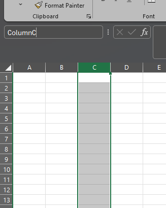
In the Excel GUI a user can define so-called Named Ranges. This is simply a range on a sheet that can be given a (meaningful) name. The easiest way of defining a name for a range in the GUI is by selecting the range you want to name and to type the name in the adress box. In the screenshot below I selected column C and gave it a name 'ColumnC'.
Now you can start using this name in formulas, like =SUM(ColumnC). This can be easier to read. Of course, these Named Ranges can also be manipulated in the VBA. This gives an elegant way of interfacing between VBA and Excel. In VBA you can use Range("ColumnC") to work with the Named Range. The advantage is also that if the named range moves on the sheet, excel will automatically update the address of the named ranges involved. So you can still use Range("ColumnC") if the range has moved.
Using VBA to manipulate Named Ranges is especially useful if the Named Range has to be dynamic. For instance when a list changes in length and you want to have a named range covering all rows.
To create a named range in VBA you can use: ActiveWorkbook.Names.Add Name:="rngName", RefersTo:="=Sheet1!$B$3:$C$4". Do not forget to include the sheet, otherwise the named range will point to the current active sheet. A named range created this way always has 'workbook' scope. Meaning you can also refer to it in formulas on other sheets then where it is defined.
To change the size of a named range in VBA you can use: Range(rngName).Resize(nrRows).Name = rngName. This will resize the named range. The top left cell will always remain the same. Only the number of rows is changed.
Likewise you can also change the nr of columns in a range with: Range(rngName).Resize(,nrCols).Name = rngName. So just leave out the row nr.
Or if you want to change both rows and columns you can use: Range(rngName).Resize(nrRows,nrCols).Name = rngName. The left top cell will remain in place. Nr of columns to the right is changed.
If you refer to a named range in VBA and it does not exist then you will get a runtime error. To prevent this you can use the following:
On Error Resume Next
ActiveWorkbook.Names.Item(rngName).RefersTo = RngAddr
' if error then Named Range did not exist yet, so create it ...
If (ERR.Number <> 0) Then ActiveWorkbook.Names.Add Name:=rngName, RefersTo:=RngAddr
On Error GoTo 0
ActiveWorkbook.Names.Item(rngName).Comment = "VBA generated"
I always like to mark the named range with the text 'VBA generated'. This way you can see in the GUI what named ranges are created by the VBA.
Note: With the new excel dynamic array formulas that use a so-called spill range the size of this resulting spill range can vary. In the excel formulas, you can refer to the entire spill range using the # after the top left cell in a formula. For instance =SUM(B3#), where B3 is the top left cell of a spill range. When no spill range exist in B3# this will just refer to B3. But you cannot use the # in VBA code to refer to the entire spill range. In VBA code you can use Range("B3").SpillingToRange to refer to the entire spill range of an dynamic array formula. If there is no spill range in the cell B3 then the result is nill.
Note: Use cannot use VBA to create or manipulate a named range that spans across sheets. This is only possible using the GUI.